
Control systems · In the CV
Adaptive Cruise Control with Lane Change
Built a cruise controller that keeps a safe gap to the car ahead and changes lanes smoothly.
- MATLAB
- Simulink
About
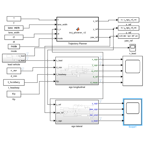
MATLAB code and a Simulink model of an adaptive cruise control (ACC) system that keeps a safe distance from a lead vehicle and performs smooth lane keeping or lane changes. A trajectory planner works with longitudinal and lateral controllers to regulate speed, steering and path tracking.
How to run
- MATLAB: keep the two .m files in one folder and run cruisecontrol.m.
- Simulink: keep the .slx model and the .mat file in one folder and run the model; it is the same ACC as the code version.
- In either case, choose the input parameters first. The files open in MATLAB R2023b or newer.
Simulink model
Source code
cruisecontrol.m
clc; clear; close all;

%% ================= User Inputs =================
T = input("Enter lane change duration [s] (default 5): ");
if isempty(T), T = 5; end

dt = input("Enter simulation time step [s] (default 0.1): ");
if isempty(dt), dt = 0.1; end

v_ego0 = input("Enter initial ego speed [m/s] (default 15): ");
if isempty(v_ego0), v_ego0 = 15; end

lane_width = input("Enter lane width [m] (default 3.5): ");
if isempty(lane_width), lane_width = 3.5; end

current_point = [0 0];   % Ego starts at origin

% Mode selection
mode = input("Choose mode: 1 = Lane Keeping, 2 = Lane Change (default 2): ");
if isempty(mode), mode = 2; end

% Lead vehicle parameters
v_lead0 = input("Enter lead vehicle initial speed [m/s] (default 13): ");
if isempty(v_lead0), v_lead0 = 13; end

x_lead0 = input("Enter initial lead vehicle X position [m] (default 30): ");
if isempty(x_lead0), x_lead0 = 30; end
y_lead = 0;   % Same lane initially

% Define multiple phases of lead vehicle motion
n_phases = input("Enter number of lead vehicle phases (default 2): ");
if isempty(n_phases), n_phases = 2; end

lead_phases = zeros(n_phases,3);
% Columns: [start_time, accel, duration]
disp("Define each phase as: start_time [s], acceleration [m/s^2], duration [s]");

for i = 1:n_phases
    fprintf("Phase %d:\n",i);
    lead_phases(i,1) = input("  Start time [s]: ");
    lead_phases(i,2) = input("  Acceleration [m/s^2] (0 = const speed, neg = braking, pos = accel): ");
    lead_phases(i,3) = input("  Duration [s]: ");
end

% ACC parameters
d_min = input("Enter minimum safe distance [m] (default 5): ");
if isempty(d_min), d_min = 5; end

t_headway = input("Enter safe time headway [s] (default 1.2): ");
if isempty(t_headway), t_headway = 1.2; end

Kp = input("Enter proportional gain Kp (default 0.5): ");
if isempty(Kp), Kp = 0.5; end

%% ================= Trajectory Planning =================
if mode == 2
    % Lane change trajectory
    [state_x,state_y,yaw_angle] = traj_planner_v2(current_point,T,v_ego0,lane_width);
else
    % Lane keeping (straight line, no y displacement)
    t_vec = 0:dt:T;
    x = current_point(1) + v_ego0*t_vec;
    state_x = [x; v_ego0*ones(size(t_vec)); zeros(size(t_vec))];
    state_y = [zeros(size(t_vec)); zeros(size(t_vec)); zeros(size(t_vec))];
    yaw_angle = zeros(size(t_vec));
end

%% ================= Simulation =================
N = length(state_x);
x_ego = state_x(1,:);
y_ego = state_y(1,:);
v_ego_profile = zeros(1,N);
x_lead_traj = zeros(1,N);
v_lead_profile = zeros(1,N);

v_ego = v_ego0;
x_lead = x_lead0;
v_lead = v_lead0;

t = (0:N-1)*dt;

for k = 1:N
    % Check current phase of lead vehicle
    a_lead = 0; % default
    for i = 1:n_phases
        if t(k) >= lead_phases(i,1) && t(k) < lead_phases(i,1) + lead_phases(i,3)
            a_lead = lead_phases(i,2);
        end
    end

    % Lead vehicle motion update
    v_lead = max(0, v_lead + a_lead*dt);   % prevent negative speed
    x_lead = x_lead + v_lead*dt;

    % Store lead vehicle data
    x_lead_traj(k) = x_lead;
    v_lead_profile(k) = v_lead;

    % Relative distance
    d_rel = x_lead - x_ego(k);
    d_safe = d_min + t_headway*v_ego;

    % ACC control law
    acc_cmd = Kp * (d_rel - d_safe);
    v_ego = max(0, v_ego + acc_cmd*dt);   % prevent negative speed

    % Store ego velocity profile
    v_ego_profile(k) = v_ego;
end

%% ================= Visualization =================
figure;

subplot(3,1,1);
plot(x_ego,y_ego,'b','LineWidth',1.5); hold on;
plot(x_lead_traj,y_lead*ones(size(t)),'r--','LineWidth',1.2); % Lead car trajectory
xlabel("X [m]"); ylabel("Y [m]");
legend("Ego trajectory","Lead car");
if mode==2
    title("Lane Change with Lead Car");
else
    title("Lane Keeping with Lead Car");
end

subplot(3,1,2);
plot(t,v_ego_profile,'b','LineWidth',1.5); hold on;
plot(t,v_lead_profile,'r--','LineWidth',1.5);
xlabel("Time [s]"); ylabel("Velocity [m/s]");
legend("Ego speed","Lead speed");
title("ACC Velocity Profile");

subplot(3,1,3);
plot(t,(x_lead_traj - x_ego),'k','LineWidth',1.5);
xlabel("Time [s]"); ylabel("Distance [m]");
title("Distance to Lead Car");
yline(d_min,'r--','Min safe distance');
traj_planner_v2.m
function [state_x,state_y,yaw_angle]=traj_planner_v2(current_point,T,v_x,lane_width)
%% Inputs:

% current_point : a 1x2 array that represents vehicle's location at the
%beginning of the lane-switching trajectory

% T : total duration of the lane change trajectory

% v_x : initial longitudinal speed at the beginning of the lane-switching

% lane_width : is the distance between adjacent lane centerline


%% Waypoint generation
% frequency = 10;%Number of commands per sec (obsolete)
dt = 0.1;

x_f = current_point(1,1) + T*v_x; % Final x coordinate
y_f = current_point(1,2) + lane_width; % Final y coordinate

%% Vehicle states in x direction (Longitudinal)
x=[];
x_dot=[];
x_ddot=[];

for t=0:dt:T
x=[x, current_point(1,1) + t*v_x];
x_dot=[x_dot,v_x];
x_ddot=[x_ddot,0];
end
state_x=[x;x_dot;x_ddot];

%%  Minimun jerk trajectory function for the calculation in y direction (Lateral)
a0=current_point(1,2);
a1=0;
a2=0;
syms a3 a4 a5;
[a3,a4,a5]=solve([a0+a3*T^3+a4*T^4+a5*T^5==y_f, ... % Boundary condition for lateral displacement
    3*a3*T^2+4*a4*T^3+5*a5*T^4==0, ...              % Boundary condition for lateral speed
    6*a3*T+12*a4*T^2+20*a5*T^3==0,],[a3,a4,a5]);    % Boundary condition for lateral acceleration

% Solving for coefficients and conversion to double precision
a3=double(a3);
a4=double(a4);
a5=double(a5);

%% Vehicle states in y direction
y=[];
y_dot=[];
y_ddot=[];
for t=0:dt:T
y=[y,a0+a1*t+a2*t^2+a3*t^3+a4*t^4+a5*t^5];
y_dot=[y_dot,a1+2*a2*t+3*a3*t^2+4*a4*t^3+5*a5*t^4];
y_ddot=[y_ddot,2*a2+6*a3*t+12*a4*t^2+20*a5*t^3];
end
state_y=[y;y_dot;y_ddot];

%% Calculate yaw angle kinematically
yaw_angle=zeros(length(x_dot),1); % Memory preallocation

for t=1:length(x_dot)
    yaw_angle(t)=atan(y_dot(t)/ (x_dot(t)));
end
%% Visualization of the Minimum Jerk Optimal Trajectory
%1. Position
figure
t=0:dt:T;
subplot(4,1,1);
plot(state_x(1,:),state_y(1,:));
legend('pos');
title("Minimum jerk trajectory");
xlabel("x direction[m]");
ylabel("y direction[m]");

%2. Velocity
subplot(4,1,2);
plot(t,state_x(2,:))
hold on;
plot(t, state_y(2,:));
legend('v_x','v_y');
title("Velocity");
xlabel("time[s]");
ylabel("Velocity[m/s]");

%3. Acceleration
subplot(4,1,3);
plot(t, state_x(3,:));
hold on;
plot(t, state_y(3,:));
legend('a_x','a_y');
title("Acceleration");
xlabel("time[s]");
ylabel("acceleration[m/s^2]");

%4. Yaw angle
subplot(4,1,4);
plot(t, yaw_angle);
hold on;
plot(t, yaw_angle);
legend('yaw angle');
title("yaw angle");
xlabel("time[s]");
ylabel("yaw angle[rad]");
end